Wearable Foot–Ankle Orthosis

Over a million people suffer ankle injuries in the U.S. each year, and roughly 30% of those are serious enough to require surgery. The problem compounds: once someone has had a serious ankle injury, an imbalanced load on that same ankle — a “bad step” — makes re-injury likely, and second injuries can take far longer to heal, sometimes permanently.

This project builds toward a wearable orthosis that gives haptic feedback the moment it senses an unsafe load. Getting there needs two things: reliably recognising what the leg is doing, and seeing a bad step coming before it lands. This page covers the sensing hardware and the deep learning work behind both.

The wearable device

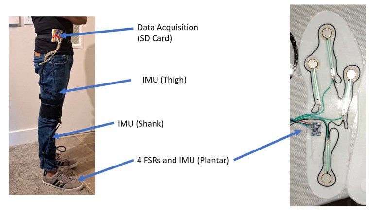
Wearable orthosis device worn on a leg, with labelled IMUs on thigh, shank and plantar section and four force-sensitive resistors under the foot — The wearable data-collection device: three IMUs on thigh, shank and plantar section, four force-sensitive resistors under the foot, logging to an SD card.

The rig captures one lower extremity through two complementary sensing modes:

4 force-sensitive resistors in the plantar region — under the 1st metatarsal, the toe, the 4th metatarsal, and the heel
3 IMUs mounted on the thigh, shank and plantar section, each contributing 3-axis gyroscope and 3-axis accelerometer readings

That gives a 22-feature vector per sample: 4 pressure values plus 3 × (3 gyro + 3 accel).

This matters because the conventional alternative is force-sensing mats and motion-capture cameras, which pin the subject to a lab, cost a great deal, and only analyse gait offline. A wearable moves the analysis online, which is the whole point if the goal is to intervene before an injury.

Data

About 40,000 samples at 24 Hz, split roughly evenly between two classes — walking and standing still — used to train the models to tell an actual step from incidental limb movement.

The raw stream was then sliced by hand so each frame holds one complete gait cycle, giving 1,944 frames (944 step, 1,000 not-step).

Frame length is the awkward part. A gait cycle’s duration depends on cadence, so frames are naturally uneven:

FCNs and CNNs need fixed-shape input, so frames were zero-padded to a common length.
RNNs and LSTMs are input-size agnostic, but PyTorch’s data loader still stacks samples, so a custom collate_fn recorded each sequence’s true length, padded to the longest frame in the set, then stripped the meaningless padding back out before the model saw it. Left in, those zeros measurably hurt learning.

Comparing four architectures

Four architectures were implemented in PyTorch and trained on the same task — is this movement a step, or not?

Model	Configuration	Learnable params	Max test accuracy
FCN	2 linear layers, ReLU, dropout(0.5)	97,132	99.9%
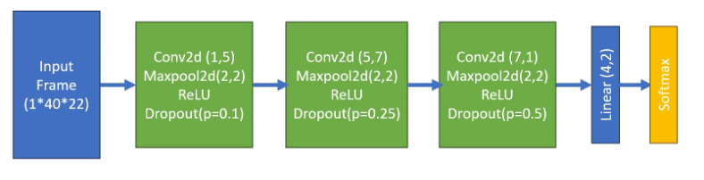
CNN	3 conv layers, 2×2 maxpool, dropout	211	95.03%
Vanilla RNN	1 layer, hidden dim 32	1,870	99.30%
LSTM	1 layer, unidirectional, hidden dim 8	7,234	99.50%

All four trained for 20 epochs with cross-entropy loss, the Adam optimiser and an 80/20 split.

The interesting result is not the top accuracy — it is the cost of that accuracy. The FCN reaches 99.9%, but needs 97,132 parameters to do it. The CNN gets to 95.03% with 211 — roughly 460× smaller, because weight sharing plus deliberately tiny 2×2 kernels keep it compact. On a device meant to run off an Arduino or Raspberry Pi, that trade is worth taking seriously.

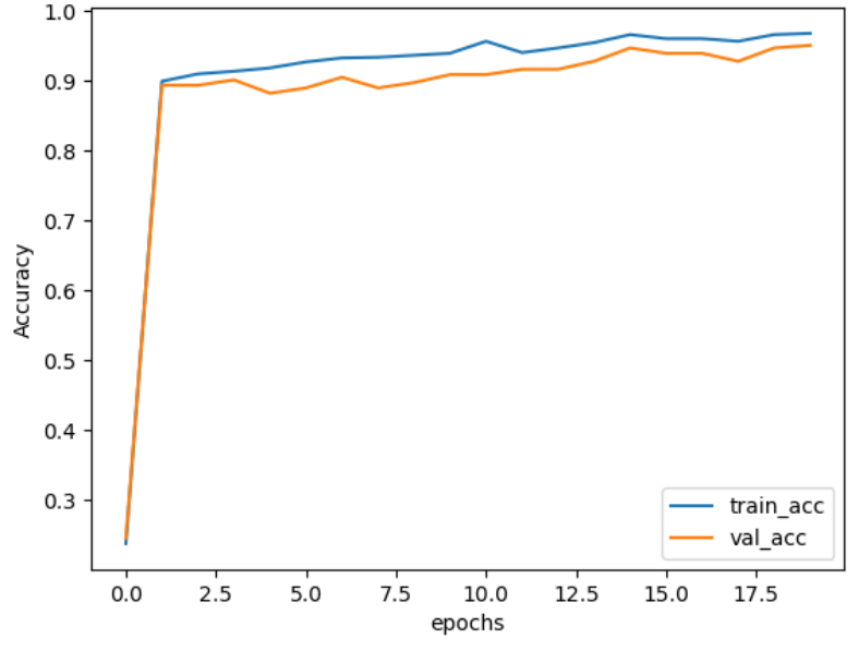
Block diagram of the CNN: input frame, three convolutional blocks with maxpool and dropout, linear layer, softmax — CNN architecture: three convolutional blocks, each with 2×2 maxpool, ReLU and dropout, feeding a linear layer and softmax.

Line chart of CNN training and validation accuracy rising to about 0.95 over 20 epochs — Training and validation accuracy for the CNN over 20 epochs.

The recurring failure mode across FCNs and CNNs was overfitting — strong on training data, weak on unseen data — handled with dropout after each layer. The FCNs also turned out to be very sensitive to input scale, which makes normalisation essential when the input mixes sensor types with different units. The vanilla RNN brought the classic problem instead: vanishing and exploding gradients, with observed loss values swinging from 40,000 down to 0.0 in floating point.

Predicting the next step

Classification alone cannot prevent an injury — by the time a bad step is classified, it has already happened. So the second half of the work asks whether the next movement can be predicted.

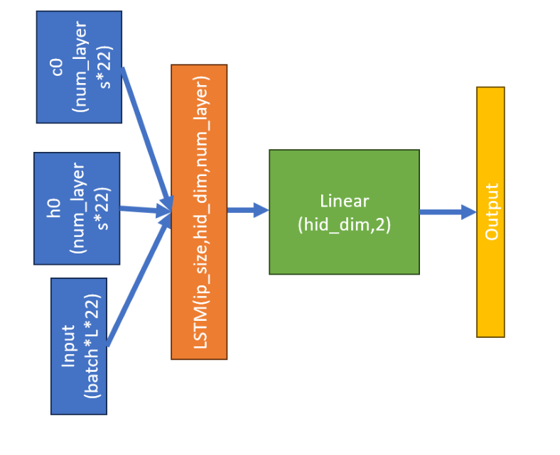
Block diagram of the LSTM model showing hidden and cell state inputs feeding an LSTM layer and a linear output layer — Condensed LSTM architecture used for the forecasting task.

This uses the LSTM in a many-to-one configuration: given the feature vectors from the previous n time steps, predict the feature vector at the current one. A look_back hyperparameter sets that window — at look_back = 30, the model sees samples t-1 through t-30 and predicts t.

Since predicting a continuous next value is closer to regression than classification, the loss is MSE. On the test set the final loss reached 0.016 — low enough to be credible for a healthcare application, on a model of only 1,222 parameters.

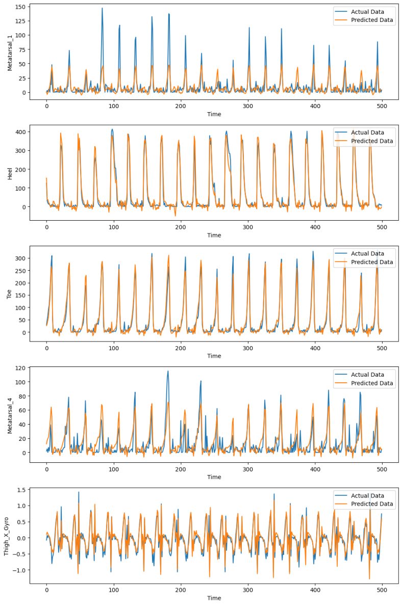
Five stacked time-series plots comparing predicted and actual sensor readings — Predicted versus actual sensor readings for the first 5 of 22 features.

Adding layers or widening the hidden dimension let the model learn more complex trends, but raised parameter count and training time — and pushed it toward memorising the training data.

Where this goes next

The target is a closed sensing-and-feedback loop running entirely on the wearable, which means shrinking the models further:

Convolutional kernel separation — splitting the standard convolution into per-channel operations to cut parameters and computation, following Bhattacharya and Lane’s work on constrained-resource inference for wearables
TensorFlow Lite — converting trained models into a form deployable on mobile and edge hardware
Extending data collection beyond walking and standing to running, jumping and other gaits, and on to labelling genuine bad steps

Inference time is the binding constraint. A prediction that arrives after the step has landed is of no use, so the real measure of success is an accurate model that is also fast enough to warn the wearer in time.